The Open Computer Vision Library known as OpenCV for short is very popular among Machine Learning engineers and Data Scientists. There are many reasons for this, but the major one is that OpenCV makes it easy to get started with working on challenging Computer Vision tasks.
As a Python developer, this crash course will equip you with enough knowledge to get started. You will learn how to:
- Install OpenCV
- Work with Images & Windows in OpenCV
- Edit Images with OpenCV
- Work with Videos in OpenCV
At the end of the article, you’ll be skilled enough to work with images and videos, and be able to work on image processing, computer vision tasks or even build your own photoshop with basic features by combining with a GUI library!
Installing OpenCV
Python, Java, and C++ are some of the languages with an OpenCV library, but this article will look into Python’s OpenCV.
OpenCV is cross platform, but you’ll need to have Python installed on your computer to get started. For Linux and Mac OS users, Python comes with the OS by default, so you do not have to bother about getting it installed. For Windows users, you’ll need to download and install the executable from the official Python Site.
Tip: Do not forget to tick the “Add to Path” directive you get when installing Python to make it easier to access it from the Command Prompt.
Open the terminal or command prompt and type in:
The command above will activate the interactive shell, which indicates a successful installation process.
Next step is to install the OpenCV and Numpy libraries; the Numpy library will come in handy at some point in this crash course.
The pip command below can help with installing both libraries:
OpenCV may have installation issues, but the command above should do the magic and install both libraries. You can import OpenCV and Numpy in the interactive shell to confirm a successful installation process.
[GCC 8.2.0] on linux
Type “help”, “copyright”, “credits” or “license” for more information.
>>> import numpy
You can move on with the rest of this crash course if you do not face any error, the show is about to get started.
Working with Images & Windows in OpenCV
Windows are the fundamentals of OpenCV as a lot of tasks depend on creating windows. In this section, you’ll learn how to create, display and destroy windows. You’ll also see how to work with images too.
Here are the things to be looked at in this section
- Creating Windows
- Displaying Windows
- Destroying Windows
- Resizing Windows
- Reading Images
- Displaying Images
- Saving Images
The code samples and images used in this section can be found on the Github repository.
Creating Windows
You’ll create windows almost every time when working with OpenCV, one of such reasons is to display images. As you’ll come to see, to display an image on OpenCV, you’ll need to create a window first, then display the image through that window.
When creating a window, you’ll use OpenCV’s namedWindow method. The namedWindow method requires you to pass in a window name of your choice and a flag; the flag determines the nature of the window you want to create.
The second flag can be one of the following:
- WINDOW_NORMAL: The WINDOW_NORMAL flag creates a window that can be manually adjustable or resizeable.
- WINDOW_AUTOSIZE: The WINDOW_AUTOSIZE flag creates a window that can’t be manually adjustable or resizeable. OpenCV automatically sets the size of the window in this case and prevents you from changing it.
There are three flags you can use for the OpenCV window, but the two above remain the most popular, and you’d often not find a use for the third.
Here’s how you call the namedWindow method:
Here’s an example:
cv2.namedWindow('Autosize', cv2.WINDOW_AUTOSIZE)
The example above will create a resizable window with the name “Normal,” and an unresizable window with the name “Autosize.” However, you won’t get to see any window displaying; this is because simply creating a window doesn’t get it to display automatically, you’ll see how to display a window in the next section.
Displaying Windows
Just as there’s no point creating a variable if you won’t be using it, there’s no point creating a window too, if you won’t be displaying it. To display the window, you’ll need OpenCV’s waitKey method. The waitKey method requires you to pass in the duration for displaying the window, which is in milliseconds.
In essence, the waitKey method displays the window for a certain duration waiting for a key to be pressed, after which it closes the window.
Here’s how you call the waitKey method:
Here’s an example:
cv2.waitKey(5000)
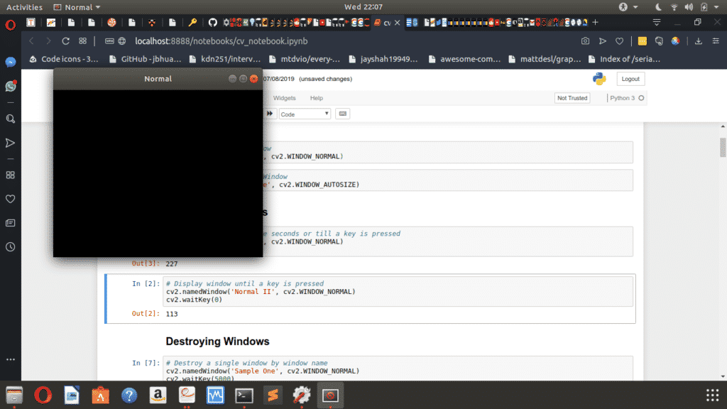
cv2.namedWindow('Normal II', cv2.WINDOW_NORMAL)
cv2.waitKey(0)
When you run the code sample above, you’ll see that it creates a window called “Normal”, which deactivates after five seconds; then it creates a window called “Normal II” and something strange happens.
The “Normal II” window refuses to close. This behavior is due to the use of the argument value 0 which causes the window to stay up “forever” until a key is pressed. Pressing a key causes the waitKey method to immediately return the integer which represents the Unicode code point of the character pressed, so it doesn’t have to wait till the specified time.
Gotcha: When the waitKey method times out or returns a value, the window becomes inactive, but it doesn’t get destroyed; so you’ll still see it on your screen. In the next section, you’ll see how to close a window after it becomes inactive.
Destroying Windows
To completely close a window, you’ll need to destroy it, and OpenCV provides the destroyWindow and destroyAllWindows methods which can help with this, though with different use cases.
You’ll use the destroyWindow to close a specific window as the method requires you to pass in the name of the window you intend destroying as a string argument. On the other hand, you’ll use the destroyAllWindows method to close all windows, and the method doesn’t take in any argument as it destroys all open windows.
Here’s how you call both methods:
cv2.destroyAllWindows()
Here’s an example:
cv2.waitKey(5000)
cv2.destroyWindow('Sample One')
cv2.namedWindow('Sample Two', cv2.WINDOW_AUTOSIZE)
cv2.namedWindow('Sample Three', cv2.WINDOW_NORMAL)
cv2.waitKey(5000)
cv2.destroyAllWindows()
When you run the code sample above, it will create and display a window named “Sample One” which will be active for 5 seconds before the destroyWindow method destroys it.
After that, OpenCV will create two new windows: “Sample Two” and “Sample Three.” Both windows are active for 5 seconds before the destroyAllWindows method destroys both of them.
To mention it again, you can also get to close the window by pressing any button; this deactivates the window in display and calls the next destroy method to close it.
Tip: When you have multiple windows open and want to destroy all of them, the destroyAllWindows method will be a better option than the destroyWindow method.
Resizing Windows
While you can pass in the WINDOW_NORMAL attribute as a flag when creating a window, so you can resize it using the mouse; you can also set the size of the window to a specific dimension through code.
When resizing a window, you’ll use OpenCV’s resizeWindow method. The resizeWindow method requires you to pass in the name of the window to be resized, and the x and y dimensions of the window.
Here’s how you call the resizeWindow method:
Here’s an example:
cv2.resizeWindow('image', 600, 300)
cv2.waitKey(5000)
cv2.destroyAllWindows()
The example will create a window with the name “image,” which is automatically sized by OpenCV due to the WINDOW_AUTOSIZE attribute. The resizeWindow method then resizes the window to a 600-by-300 dimension before the window closes five seconds after.
Reading Images
One key reason you’ll find people using the OpenCV library is to work on images and videos. So in this section, you’ll begin to see how to do that and the first step will be reading images.
When reading images, you’ll use OpenCV’s imread method. The imread method requires you to pass in the path to the image file as a string; it then returns the pixel values that make up the image as a 2D or 3D Numpy array.
Here’s how you call the imread method:
Here’s an example:
print(image)
The code above will read the “testimage.jpg” file from the “images” directory, then print out the Numpy array that makes up the image. In this case, the image is a 3D array. It’s a 3D array because OpenCV reads images in three channels (Blue, Green, Red) by default.
The Numpy array gotten from the image takes a format similar to this:
[255 204 0]
[255 204 0]
...,
[255 204 0]
[255 204 0]
[255 204 0]]
...
Gotcha: Always ensure to pass the right file path into the imread method. OpenCV doesn’t raise errors when you pass in the wrong file path, instead it returns a None data type.
While the imread method works fine with only one argument, which is the name of the file, you can also pass in a second argument. The second argument will determine the color mode OpenCV reads the image in.
To read the image as Grayscale instead of BGR, you’ll pass in the value 0. Fortunately, OpenCV provides an IMREAD_GRAYSCALE attribute that you can use instead.
Here’s an example:
print(image)
The code above will read the “testimage.jpg” file in Grayscale mode, and print the Numpy array that makes up the image.
The result will take a format similar to this:
[149 149 149 ..., 149 149 149]
[149 149 149 ..., 149 149 149]
...,
[149 149 149 ..., 148 148 149]
[149 149 149 ..., 148 148 149]
[149 149 149 ..., 148 148 149]]
The Numpy array you’ll get from reading an image in Grayscale mode is a 2D array; this is because Grayscale images have only one channel compared to three channels from BGR images.
Displaying Images
All this while, you’ve created windows without images in them; now that you can read an image using OpenCV, it’s time to display images through the windows you create.
When displaying images, you’ll use OpenCV’s imshow method. The imshow method requires the name of the window for displaying the image, and the Numpy array for the image.
Here’s how you call the imshow method:
Here’s an example:
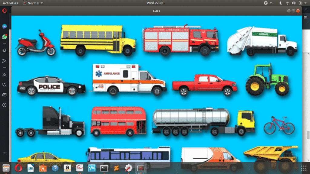
cv2.namedWindow('Cars', cv2.WINDOW_NORMAL)
cv2.imshow('Cars', image)
cv2.waitKey(5000)
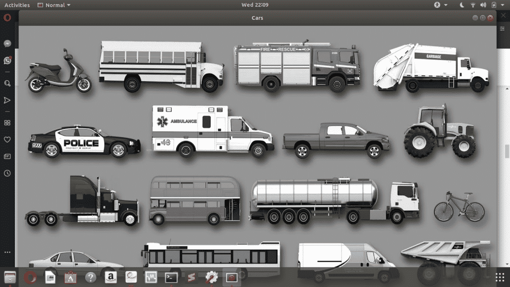
image = cv2.imread('./images/testimage.jpg', cv2.IMREAD_GRAYSCALE)
cv2.imshow('Cars', image)
cv2.waitKey(5000)
cv2.destroyWindow('Cars')
The code sample above will read the image, create a window named “Cars” and display the image through the window for five seconds using the imshow method. When the 5-second limit elapses, OpenCV will read the image again but this time in Grayscale mode; the same window displays the Grayscale image for five seconds then closes.
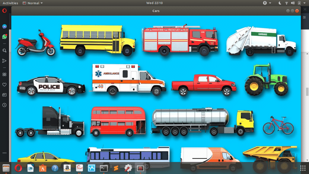
Image of Cars
Saving Images
In the latter part of this crash course, you’ll get to modify, add watermarks, and draw shapes on images. So you’d need to save your images so as not to lose the changes.
When saving images, you’ll use OpenCV’s imwrite method. The imwrite method requires you to pass in the path where you intend to save the image file, and the Numpy array that makes up the image you want to save.
Here’s how you call the imwrite method:
Here’s an example:
cv2.imwrite("./images/grayimage.jpg", gray_image)
The code above will read the “testimage.jpg” image in Grayscale mode, then save the Grayscale image as “grayimage.jpg” to the “images” directory. Now, you’ll have copies of the original and Grayscale image saved in storage.
Editing Images with OpenCV
It’s about time to go a bit in depth into the world of image processing with OpenCV, you’ll find the knowledge of creating windows, reading and displaying images from the previous section useful; you also need to be comfortable with working with Numpy arrays.
Here are the things to be looked at in this section
- Switching Color Modes
- Editing Pixel Values
- Joining Images
- Accessing Color Channels
- Cropping Images
- Drawing on Images
- Blurring Images
The code samples and images used in this section can be found on the Github repository.
Switching Color Modes
When processing images for tasks such as medical image processing, computer vision, and so on, you’ll often find reasons to switch between various colour modes.
You’ll use OpenCV’s cvtColor method when converting between color modes. The cvtColor method requires you to pass in the Numpy array of the image, followed by a flag that indicates what color mode you want to convert the image to.
Here’s how you call the cvtColor method:
Here’s an example:
cv2.imshow('Cars', image_mode)
cv2.waitKey(5000)
cv2.destroyAllWindows()
The code sample above will convert the image from the BGR to YCrCb color mode; this is because of the use of the integer value 36 which represents the flag for BGR to YCrCb conversions.
Here’s what you’ll get:

OpenCV provides attributes that you can use to access the integer value that corresponds to the conversion you want to make; this makes it easier to convert between different modes without memorizing the integer values.
Here are some of them:
- COLOR_RGB2GRAY: The COLOR_RGB2GRAY attribute is used to convert from the RGB color mode to Grayscale color mode.
- COLOR_RGB2BGR: The COLOR_RGB2BGR attribute is used to convert from the RGB color mode to BGR color mode.
- COLOR_RGB2HSV: The COLOR_RGB2HSV attribute is used to convert from the RGB color mode to HSV color mode.
Here’s an example that converts an image from the RGB to Grayscale color mode
image_gray = cv2.cvtColor(image, cv2.COLOR_BGR2GRAY)
cv2.imshow('Cars', image_gray)
cv2.waitKey(5000)
cv2.destroyAllWindows
The code sample above will read the image using the imread method, then convert it from the default BGR to Grayscale mode before displaying the image for 5 seconds.
Here’s the result:
A Grayscale Image of Cars
Editing Pixel Values
Images are made up of picture elements known as pixels, and every pixel has a value that gives it color, based on the colour mode or channel. To make edits to an image, you need to alter its pixel values.
There is no specific method for editing pixel values in OpenCV; however, since OpenCV reads the images as Numpy arrays, you can replace the pixel values at different positions in the array to get the desired effect.
To do this, you need to know the image’s dimensions and number of channels; these can be gotten through the shape attribute.
Here’s an example:
print(image.shape)
The code sample above will yield the result:
From the result, you can see that the image has a 720 (height) by 1280 (width) dimension and three channels. Don’t forget that OpenCV reads image by default as a BGR (Blue, Green and Read) channel.
Here’s a second example:
print(image_gray.shape)
The code sample above will yield the result:
From the result, you can see that the image has a 720 (height) by 1280 (width) dimension and it has one channel. The image has only one channel because the first line of code reads the image as a Grayscale image. Grayscale images have only one channel.
Now that you have an idea of the image’s properties by dimension and channels, you can alter the pixels.
Here’s a code sample:
edited_image = image.copy()
edited_image[:, :640] = 0
cv2.namedWindow('Cars',cv2.WINDOW_NORMAL)
cv2.imshow('Cars', edited_image)
cv2.waitKey(5000)
cv2.destroyWindow('Cars')
The code sample above makes the left half of the image black. When you learn about colour modes, you’ll see that the value 0 means black, while 255 means white with the values in-between being different shades of grey.
Here’s the result:
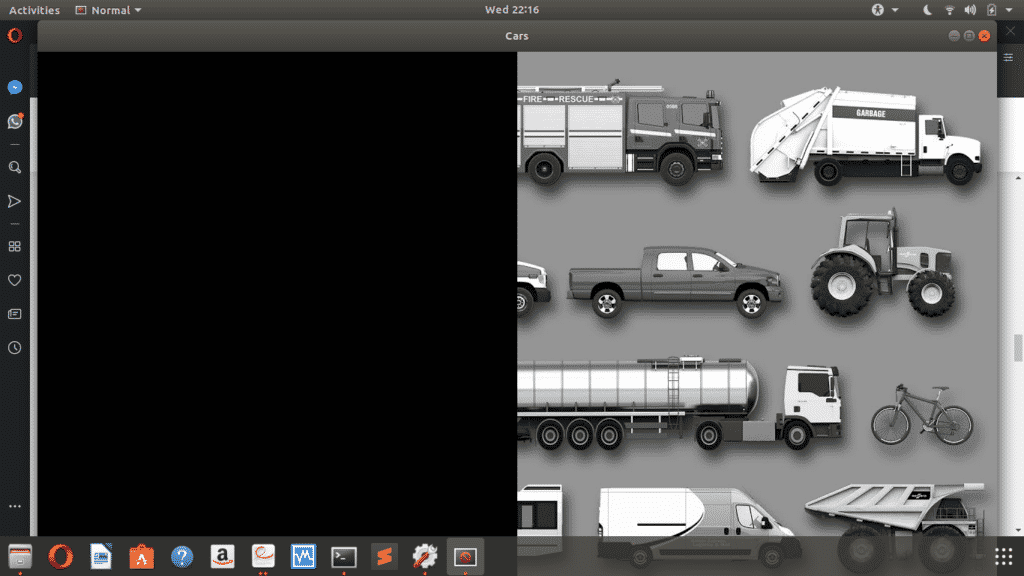
Left Side of Image Filled With Black
Since the image has a 720-by-1280 dimension, the code makes half of the pixels in the x-axis zero (from index 0 to 640), which has an effect of turning all pixels in that region black.
Gotcha: OpenCV reads images as columns first, then rows instead of the conventional rows before columns, so you should watch out for that.
The use of the copy method is to ensure that OpenCV copies the image object into another variable. It is important to copy an image because when you make changes to the original image variable, you can’t recover its image values.
In summary, the concept of editing pixel values involves assigning new values to the pixels to achieve the desired effect.
Joining Images
Have you ever seen an image collage? With different images placed side by side. If you have, then you’d have a better understanding of the need to join images.
OpenCV doesn’t provide methods that you can use to join images. However, the Numpy library will come in handy in this scenario.
Numpy provides the hstack and vstack methods which you can use to stack arrays side by side horizontally or vertically.
Here’s how you call both methods:
np.vstack((image1, image2, ..., imagen))
Here’s an example of both in action:
hcombine = np.hstack((image, image, image))
cv2.imshow("Cars Combined", hcombine)
cv2.waitKey(5000)
vcombine = np.vstack((image, image, image))
cv2.imshow("Cars Combined", vcombine)
cv2.waitKey(5000)
cv2.destroyAllWindows()
The code sample above will read the image, join (stack) the resulting Numpy array horizontally in three places, then display it for five seconds. The second section of the code sample joins (stacks) the image array from the first section vertically in three places and displays it too.
Here’s the result:
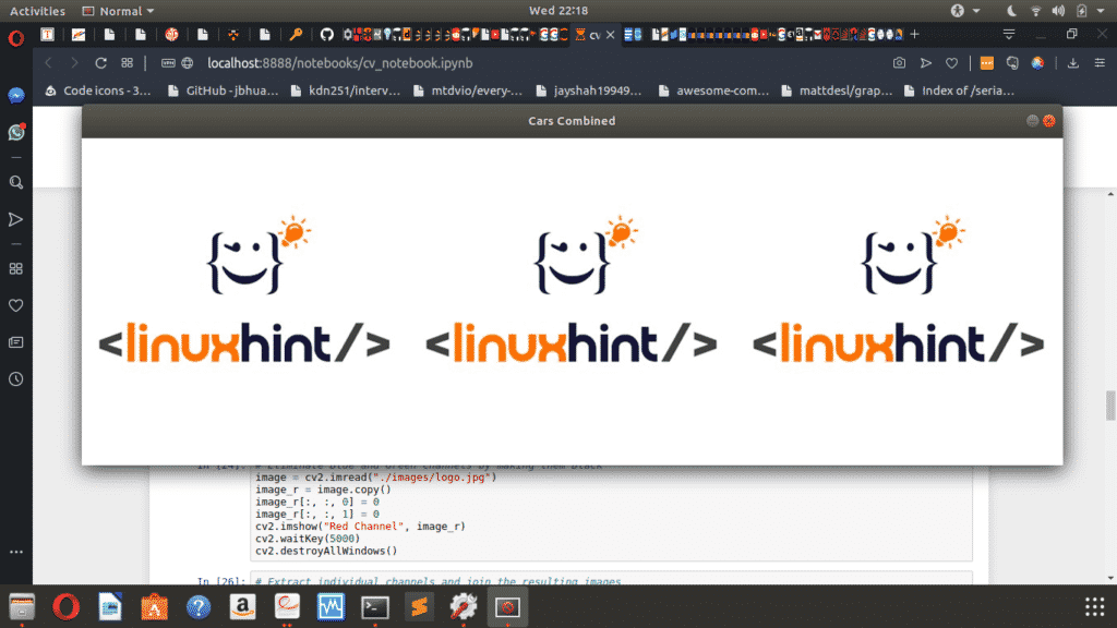
Horizontal Stack of Three Images
Accessing Color Channels
In the last two sections, the concept of joining images and editing image pixel values (for Grayscale images) was viewed. However, it may be a bit complex when the image has three channels instead of one.
When it comes to images with three channels, you can access the pixel values of individual colour channels. While OpenCV doesn’t provide a method to do this, you’ll find it to be an easy task with an understanding of Numpy arrays.
When you read an image having three channels, the resulting numpy array is a 3D numpy array. So one way to go about viewing individual channels is to set the other channels to zero.
So you can view the following channels by:
- Red channel: Setting the Blue and Green channels to zero.
- Blue channel: Setting the Red and Green channels to zero.
- Green channel: Setting the Red and Blue Channels to zero.
Here’s an example:
image_r[:, :, 0] = 0
image_r[:, :, 1] = 0
cv2.imshow("Red Channel", image_r)
cv2.waitKey(5000)
cv2.destroyAllWindows()
The code sample above will copy the image’s Numpy array, set the Blue and Green channel to zero, then display an image with only one active channel (the Red channel).
Here’s a code sample to display the other channels side-by-side on the same window
image_b = image.copy()
image_b[:, :, 1] = 0
image_b[:, :, 2] = 0
image_g = image.copy()
image_g[:, :, 0] = 0
image_g[:, :, 2] = 0
image_r = image.copy()
image_r[:, :, 0] = 0
image_r[:, :, 1] = 0
numpy_horizontal = np.hstack((image_b, image_g, image_r))
cv2.namedWindow('image',cv2.WINDOW_NORMAL)
cv2.resizeWindow('image', 800, 800)
cv2.imshow("image", numpy_horizontal)
cv2.waitKey(5000)
cv2.destroyAllWindows()
The code sample above reads the image, extracts the corresponding colour channels, then stacks the results horizontally before displaying to the screen.
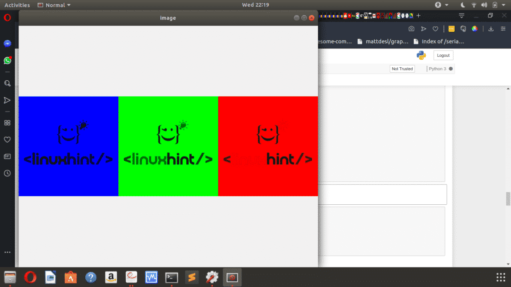
Horizontal Stack of an Image’s Blue, Green and Red Channels
Cropping Images
There are many reasons for which you may want to crop an image, but the end goal is to extract the desired aspect of the image from the complete picture. Image cropping is popular, and it’s a feature you’ll find on almost every image editing tool. The good news is that you can pull it off using OpenCV too.
To crop an image using OpenCV, the Numpy library will be needed; so an understanding of Numpy arrays will also come in handy.
The idea behind cropping images is to figure out the corners of the image you intend cropping. In the case of Numpy, you only need to figure out the top-left and bottom-right corners, then extract them using index slicing.
Going by the explanation above, you’ll be needing four values:
- X1
- X2
- Y1
- Y2
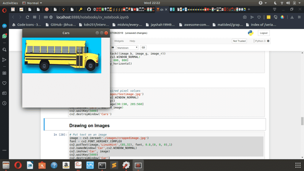
Below is a code sample to show the concept of cropping images:
cv2.namedWindow('Cars',cv2.WINDOW_NORMAL)
edited_image = image.copy()
edited_image = edited_image[30:190, 205:560]
cv2.imshow('Cars', edited_image)
cv2.waitKey(5000)
cv2.destroyWindow('Cars')
Here’s the result:
Drawing on Images
OpenCV allows you to alter images by drawing various characters on them such as inputting text, drawing circles, rectangles, spheres, and polygons. You’ll learn how to do this in the rest of this section, as OpenCV provides specific functions that will help you draw a couple of characters on images.
You’ll see how to add the following to images in this section:
- Text
- Lines
- Circles
Text
OpenCV provides the putText method for adding text to images. The putText method requires you to pass in the image’s Numpy array, the text, positioning coordinates as a tuple, the desired font, text’s size, color, and width.
Here’s how you call the putText method:
For the fonts, OpenCV provides some attributes that you can use for selecting fonts instead of memorizing the integer values.
Here are some of them:
- FONT_HERSHEY_COMPLEX
- FONT_HERSHEY_DUPLEX
- FONT_HERSHEY_PLAIN
- FONT_ITALIC
- QT_FONT_BOLD
- QT_FONT_NORMAL
You can experiment with the different font types to find the one that best suits your purpose.
Here’s a code example that adds text to an image:
font = cv2.FONT_HERSHEY_COMPLEX
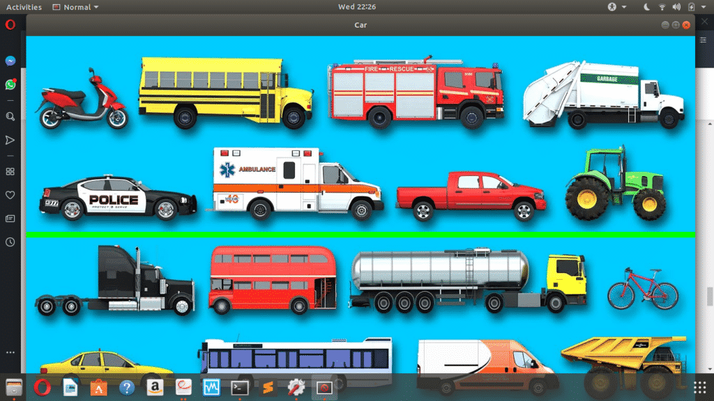
cv2.putText(image,'LinuxHint',(85,32), font, 0.8,(0, 0, 0),1)
cv2.namedWindow('Car',cv2.WINDOW_NORMAL)
cv2.imshow('Car', image)
cv2.waitKey(5000)
cv2.destroyWindow('Car')
The code above reads the passed in the image, which is the cropped image from the previous section. It then accesses the flag for the font of choice before adding the text to the image and displaying the image.
Here’s the result:
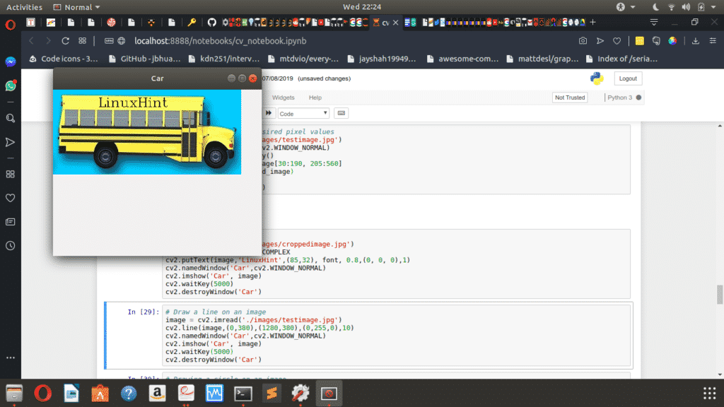
“LinuxHint” on a Vehicle
Lines
OpenCV provides the line method for drawing lines on images. The line method requires you to pass in the image’s Numpy array, positioning coordinates for the start of the line as a tuple, positioning coordinates for the end of the line as a tuple, the line’s color and thickness.
Here’s how you call the line method:
Here’s a code sample that draws a line on an image:
cv2.line(image,(0,380),(1280,380),(0,255,0),10)
cv2.namedWindow('Car',cv2.WINDOW_NORMAL)
cv2.imshow('Car', image)
cv2.waitKey(5000)
cv2.destroyWindow('Car')
The code sample above will read the image, then draw a green line on it. In the code sample’s second line, you’ll see the coordinates for the start and end of the line passed in as different tuples; you’ll also see the color and thickness.
Here’s the result:
A Green Line Drawn at The Middle of the Image
Drawing Circles
OpenCV provides the circle method for drawing circles on images. The circle method requires you to pass in the image’s Numpy array, center coordinates (as a tuple), the circle’s radius, color, and thickness.
Here’s how you call the circle method:
Tip: To draw a circle with the least thickness, you’ll pass in the value 1, on the other hand, passing in the value -1 will cover up the circle completely, so you should watch out for that.
Here’s a code sample to show the drawing of a circle on an image:
cv2.circle(image,(110,125), 100, (0,0,255), -1)
cv2.circle(image,(1180,490), 80, (0,0,0), 1)
cv2.namedWindow('Car',cv2.WINDOW_NORMAL)
cv2.imshow('Car', image)
cv2.waitKey(5000)
cv2.destroyWindow('Car')
The code sample above draws two circles on the image. The first circle has a thickness value of -1, so it has full thickness. The second has a thickness value of 1, so it has the least thickness.
Here’s the result:
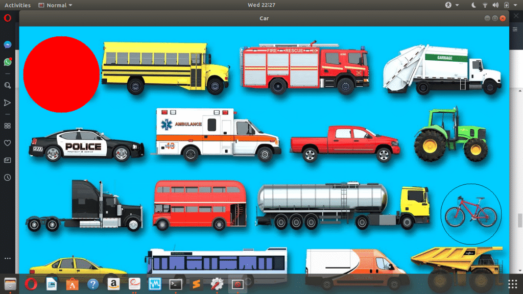
Two Circles Drawn on an Image
You can also draw other objects such as rectangles, ellipses, or polygons using OpenCV, but they all follow the same principles.
Blurring Images
So far, you’ve seen OpenCV’s ability to perform some tasks you’d find on a powerful photo-editing tool such as Photoshop on a fundamental level. That’s not all; you can also blur images using OpenCV.
OpenCV provides the GaussianBlur method, which you can use for blurring images using Gaussian Filters. To use the GaussianBlur method, you’ll need to pass in the image’s Numpy array, kernel size, and sigma value.
You don’t have to worry so much about the concept of the kernel size and sigma value. However, you should note that kernel sizes are usually in odd numbers such as 3×3, 5×5, 7×7 and the larger the kernel size, the greater the blurring effect.
The sigma value, on the other hand, is the Gaussian Standard Deviation and you’ll work fine with an integer value of 0. You may decide to learn more about the sigma value and kernels for image filters.
Here’s how you call the GaussianBlur method:
Here’s a code sample that performs the blurring of an image:
blurred = cv2.GaussianBlur(image, (5,5), 0)
cv2.namedWindow('Cars', cv2.WINDOW_NORMAL)
cv2.imshow('Cars', blurred)
cv2.waitKey(5000)
cv2.destroyWindow('Cars')
The code sample above uses a kernel size of 5×5 and here’s the result:
A Little Blurring on the Image
Tip: The larger the kernel size, the greater the blur effect on the image.
Here’s an example:
blurred = cv2.GaussianBlur(image, (25,25), 0)
cv2.namedWindow('Cars', cv2.WINDOW_NORMAL)
cv2.imshow('Cars', blurred)
cv2.waitKey(5000)
cv2.destroyWindow('Cars')
As you’ll see with the result, the image experiences more blur using a kernel size of 25×25. Here it is:
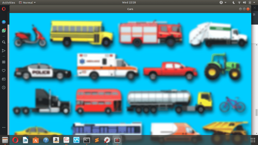
Increased Blurring on an Image
Working with Videos in OpenCV
So far, you’ve seen how powerful OpenCV can be with working with images. But, that’s just the tip of the iceberg as this is a crash course.
Moving forward, you’ll learn how to make use of OpenCV when working with videos.
Here are the things to be looked at in this section:
- Loading Videos
- Displaying Videos
- Accessing the WebCam
- Recording Videos
The same way there was a specified video for the sections when working with images, you’ll find the video for this tutorial in the “videos” directory on the GitHub repository with the name “testvideo.mp4.” However, you can make use of any video of your choice.
If you take a closer look at videos, you’ll realize they are also images with a time dimension, so most of the principles that apply to images also apply to videos.
Loading Videos
Just as with images, loading a video doesn’t mean displaying the video. However, you’ll need to load (read) the video file before you can go ahead to display it.
OpenCV provides the VideoCapture method for loading videos. The VideoCapture method requires you to pass in the path to the image and it’ll return the VideoCapture object.
Here’s how you call the VideoCapture method:
Here’s a code sample that shows how you load a video:
Gotcha: The same pitfall with loading images applies here. Always ensure to pass in the right file path as OpenCV won’t raise errors when you pass in a wrong value; however, the VideoCapture method will return None.
The code sample above should correctly load the video. After the video loads successfully, you’ll still need to do some work to get it to display, and the concept is very similar to what you’ll do when trying to display images.
Displaying Videos
Playing videos on OpenCV is almost the same as displaying images, except that you are loading images in a loop, and the waitKey method becomes essential to the entire process.
On successfully loading a video file, you can go ahead to display it. Videos are like images, but a video is made up of a lot of images that display over time. Hence, a loop will come in handy.
The VideoCapture method returns a VideoCapture object when you use it to load a video file. The VideoCapture object has an isOpened method that returns the status of the object, so you’ll know if it’s ready to use or not.
If the isOpened method returns a True value, you can proceed to read the contents of the file using the read method.
OpenCV doesn’t have a displayVideo method or something in that line to display videos, but you can work your way around using a combination of the available methods.
Here’s a code sample:
while(video.isOpened()):
ret, image = video.read()
if image is None:
break
cv2.imshow('Video Frame', image)
if cv2.waitKey(1) & 0xFF == ord('q'):
break
video.release()
cv2.destroyAllWindows()
The code sample loads the video file using the VideoCapture method, then checks if the object is ready for use with the isOpened method and creates a loop for reading the images.
The read method in the code works like the read method for reading files; it reads the image at the current position and moves to the next waiting to be called again.
In this case, the read method returns two values, the first showing the status of the attempt to read the image—True or False—and the second being the image’s array.
Going by the explanation above, when the read method gets to a point where there’s no image frame to read, it simply returns (False, None) and the break keyword gets activated. If that’s not the case, the next line of code displays the image that the read method returns.
Remember the waitKey method?
The waitKey method displays images for the number of milliseconds passed into it. In the code sample above, it’s an integer value 1, so each image frame only displays for one millisecond. The next code sample below uses the integer value 40, so each image frame displays for forty milliseconds and a lag in the video becomes visible.
The code section with 0xFF == ord(‘q’) checks if the key “q” is pressed on the keyboard while the waitKey method displays the image and breaks the loop.
The rest of the code has the release method which closes the VideoCapture object, and the destroyAllWindows method closes the windows used in displaying the images.
Here’s the code sample with the argument value of 40 passed into the waitKey method:
while(video.isOpened()):
ret, image = video.read()
if image is None:
print(ret)
break
cv2.imshow('Video Frame', image)
if cv2.waitKey(40) & 0xFF == ord('q'):
break
video.release()
cv2.destroyAllWindows()
Accessing the WebCam
So far, you’ve seen how to load a video file from your computer. However, such a video won’t display in real-time. With the webcam, you can display real-time videos from your computer’s camera.
Activating the webcam requires the VideoCapture method, which was used to load video files in the previous section. However, in this case, you will be passing the index value of the webcam into the VideoCapture method instead of a video file path.
Hence, the first webcam on your computer has the value 0, and if you have a second one, it’ll have the value 1.
Here’s a code sample below that shows how you can activate and display the contents of your computer’s webcam:
while(video.isOpened()):
ret, image = video.read()
cv2.imshow('Live Cam', image)
if cv2.waitKey(1) & 0xFF == ord('q'):
break
video.release()
cv2.destroyAllWindows()
The value 1 is used for the waitKey method because a real-time video display needs the waitKey method to have the smallest possible wait-time. Once again, to make the video display lag, increase the value passed into the waitKey method.
Recording Videos
Being able to activate your computer’s webcam allows you to make recordings, and you’ll see how to do just that in this section.
OpenCV provides the VideoWriter and VideoWriter_fourcc methods. You’ll use the VideoWriter method to write the videos to memory, and the VideoWriter_fourcc to determine the codec for compressing the frames; the codec is a 4-character code which you’ll understand better with the knowledge of codecs.
Here’s how you call the VideoWriter_fourcc method:
Here are some examples you’ll find:
cv2.VideoWriter_fourcc('X','V','I','D')
The VideoWriter method, on the other hand, receives the name you wish to save the video with, the fourcc object from using the VideoWriter_fourcc method, the video’s FPS (Frame Per Seconds) value and frame size.
Here’s how you call the VideoWriter method:
Below is a code sample that records video using the webcam and saves it as “out.avi”:
fourcc = cv2.VideoWriter_fourcc('X','V','I','D')
writer = cv2.VideoWriter('out.avi',fourcc, 15.0, (640,480))
while(video.isOpened()):
ret, image = video.read()
writer.write(image)
cv2.imshow('frame',image)
if cv2.waitKey(1) & 0xFF == ord('q'):
break
video.release()
writer.release()
cv2.destroyAllWindows()
The code sample above activates the computer’s webcam and sets up the fourcc to use the XVID codec. After that, it calls the VideoWriter method by passing in the desired arguments such as the fourcc, 15.0 for FPS and (640, 480) for the frame size.
The value 15.0 is used as FPS because it provides a realistic speed for the video recording. But you should experiment with higher or lower values to get a desirable result.
Conclusion
Congratulations on getting to the end of this crash course, you can check out the Github repository to check out the code for reference purposes. You now know how to make use of OpenCV to display images and videos, crop and edit images, create a photo collage by combining images, switch between color modes for computer vision and image processing tasks among other newly gained skills.
In this OpenCV crash course, you’ve seen how to:
- Setup the library
- Work with Images & Windows
- Edit Images
- Work with Videos
Now you can go ahead to take on advanced OpenCV tasks such as face recognition, create a GUI application for editing images or check out Sentdex’s OpenCV series on YouTube.